Basic Theoretical Information
Harmonic vibrations
In technology and the world around us, we often encounter periodic processes that repeat at regular intervals of time. Such processes are called oscillatory. Fluctuations are changes in a physical quantity that occur according to a certain law in time. Oscillatory phenomena of different physical natures obey the general laws. For example, current oscillations in an electrical circuit and oscillations of a mathematical pendulum can be described by the same equations. The generality of the oscillatory laws allows us to consider the oscillatory processes of different natures from a single point of view.
Mechanical vibrations are called the movement of bodies, repeating exactly at equal intervals of time. Examples of simple oscillatory systems include a spring-loaded load or a mathematical pendulum. For the existence of harmonic oscillations in the system, it is necessary for it to have a position of stable equilibrium, that is, a situation when removing from which a restoring force would act on the system.
Mechanical oscillations, like oscillatory processes of any other physical nature, can be free and forced. Free vibrations are made under the action of the internal forces of the system after the system has been brought out of equilibrium. The oscillations of the load on the spring or the oscillations of the pendulum are free oscillations. Oscillations occurring under the influence of external periodically changing forces are called forced.
The simplest type of oscillatory process is oscillations occurring according to the law of sine or cosine, called harmonic oscillations. The equation describing physical systems capable of performing harmonic oscillations with a cyclic frequency ω 0 is defined as follows:

The solution of the previous equation is the equation of motion for harmonic oscillations , which has the form:

where: x is the body displacement from the equilibrium position, A is the oscillation amplitude, that is, the maximum displacement from the equilibrium position, ω is the cyclic or circular oscillation frequency ( ω = 2 Π / T ), t is the time. The value under the cosine sign: φ = ωt + φ 0 is called the phase of the harmonic process. The meaning of the oscillation phase: the stage in which the oscillation is at a given time. When t = 0, we get φ = φ 0 , so φ 0called the initial phase(that is, the stage from which the oscillation began).
The minimum time interval after which repetition body motion occurs, is called the period of oscillation T . If the number of oscillations is N , and their time is t , then the period is as:

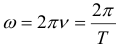
The inverse of the oscillation period is called the oscillation frequency :

The oscillation frequency ν indicates how many oscillations occur in 1 second. The unit of frequency is Hertz (Hz). The oscillation frequency is associated with the cyclic frequency ω and the oscillation period T by the relations:
The dependence of speed on time with harmonic mechanical vibrations is expressed by the following formula:

Maximum speed value with harmonic mechanical oscillations:

The maximal values of the velocity υ m = ωA are reached at those times when the body passes through equilibrium positions ( x = 0). The acceleration a = a x of the body is determined in a similar way with harmonic oscillations. The dependence of acceleration on time with harmonic mechanical vibrations:

Maximum value of acceleration with mechanical harmonic oscillations:

The minus sign in the previous expression means that the acceleration a ( t ) always has a sign opposite to the x ( t ) offset sign , and therefore returns the body to its initial position ( x = 0), i.e. causes the body to make harmonic vibrations.
It should be noted that:
- physical properties of the oscillating system is only determined natural frequency ω 0 or period T .
- Such parameters of the oscillation process, such as the amplitude A = x m and the initial phase φ 0 , are determined by the method by which the system was brought out of equilibrium at the initial time, i.e. initial conditions.
- In the case of oscillatory motion, the body travels in a time equal to a period equal to 4 amplitudes. In this case, the body returns to the starting point, that is, the movement of the body will be zero. Consequently, the path is equal to the amplitude of the body will be for a time equal to a quarter of the period.
To determine when to substitute the sine in the oscillation equation, and when cosine, you need to pay attention to the following factors:
- The easiest way is if in the condition of the problem the oscillations are called sine or cosine.
- If it is said that the body was pushed out of the equilibrium position, then we take a sine with an initial phase equal to zero.
- If it is said that the body was rejected and released, the cosine with the initial phase equal to zero.
- If the body is pushed out of a state deviated from the equilibrium state, then the initial phase is not equal to zero, and both sine and cosine can be taken.
Math Pendulum
A mathematical pendulum is a small-sized body suspended from a thin, long and inextensible filament, whose mass is negligible compared to its mass. Only in the case of small oscillations, the mathematical pendulum is a harmonic oscillator , that is, a system capable of performing harmonic (as sin or cos) oscillations. In practice, this approximation is valid for angles of the order of 5–10 °. The oscillations of the pendulum at large amplitudes are not harmonic.
The cyclic frequency of oscillations of the mathematical pendulum is calculated by the formula:

The period of oscillation of the mathematical pendulum:
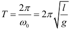
The resulting formula is called the Huygens formula and is executed when the suspension point of the pendulum is fixed . It is important to remember that the period of small oscillations of a mathematical pendulum does not depend on the amplitude of oscillations. This property of the pendulum is called isochronism . As with any other system that performs mechanical harmonic oscillations, the following relations for the mathematical pendulum are fulfilled:
- The path from the equilibrium position to the extreme point (or back) passes through a quarter of a period.
- The path from the extreme point to the half amplitude (or vice versa) is covered in one sixth of the period.
- The path from the equilibrium position to half the amplitude (or back) passes through one twelfth of the period.
Spring pendulum
Free vibrations are made under the action of the internal forces of the system after the system has been removed from the equilibrium position. In order for the free oscillations to be performed according to the harmonic law, it is necessary that the force striving to return the body to the equilibrium position be proportional to the displacement of the body from the equilibrium position and directed in the direction opposite to the displacement. This property has the strength of elasticity.
Thus, the load of a certain mass m , attached to the spring of stiffness k , the second end of which is fixed motionless, constitutes a system capable of performing free harmonic oscillations in the absence of friction. The load on the spring is called the spring pendulum .
The cyclic frequency of oscillation of the spring pendulum is calculated by the formula:

The period of oscillation of the spring pendulum:
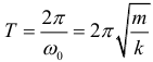
At small amplitudes, the oscillation period of the spring pendulum does not depend on the amplitude (as in the case of the mathematical pendulum). When the spring – load system is horizontal, the gravitational force applied to the load is compensated by the support reaction force. If the load is suspended on a spring, then the force of gravity is directed along the line of movement of the load. In the equilibrium position, the spring is stretched by an amount x 0 equal to:

And oscillations occur around this new equilibrium position. The above expressions for the natural frequency ω 0 and the oscillation period T are also valid in this case. Thus, the resulting formula for the period of oscillation of the load on the spring remains valid in all cases, regardless of the direction of oscillation, the movement of the support, the action of external constant forces.
With free mechanical vibrations, the kinetic and potential energies change periodically. At the maximum deviation of the body from the equilibrium position, its velocity, and, consequently, the kinetic energy, vanish. In this position, the potential energy of the oscillating body reaches its maximum value. For a load on a spring, the potential energy is the energy of the elastic deformation of the spring. For a mathematical pendulum, it is energy in the field of the Earth.
When the body during its movement passes through the equilibrium position, its speed is maximum. The body skips the equilibrium position by inertia. At this moment it has the maximum kinetic and minimum potential energy (as a rule, the potential energy in the equilibrium position is assumed to be zero). The increase in kinetic energy occurs due to a decrease in potential energy. With further movement, the potential energy begins to increase due to the loss of kinetic energy and so on.
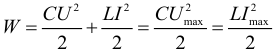
Thus, with harmonic oscillations, the kinetic energy is periodically transformed into potential energy and vice versa. If there is no friction in the oscillatory system, then the total mechanical energy with free oscillations remains unchanged. At the same time, the maximum value of the kinetic energy during mechanical harmonic oscillations is given by the formula:

The maximum value of potential energy during mechanical harmonic oscillations of a spring pendulum:

The relationship of the energy characteristics of a mechanical oscillatory process (the total mechanical energy is equal to the maximum values of the kinetic and potential energies, as well as the sum of the kinetic and potential energies at an arbitrary point in time):

Mechanical waves
If in any place of a solid, liquid or gaseous medium, oscillations of particles are excited, then due to the interaction of atoms and molecules of the medium, oscillations begin to be transferred from one point to another with a finite velocity. The process of propagation of oscillations in the medium is called a wave .
Mechanical waves are of different types. If during the propagation of a wave, the particles of the medium experience an offset in the direction perpendicular to the direction of propagation, such a wave is called transverse . If the displacement of particles of the medium occurs in the direction of wave propagation, this wave is called a longitudinal one .
In both transverse and longitudinal waves, there is no transfer of matter in the direction of wave propagation. In the process of propagation, particles of the medium only oscillate around equilibrium positions. However, waves transfer vibrational energy from one point of the medium to another.
A characteristic feature of mechanical waves is that they propagate in material media (solid, liquid or gaseous). There are non-mechanical waves that can propagate in a vacuum (for example, light, that is, electromagnetic waves can propagate in a vacuum).
- Longitudinal mechanical waves can propagate in any medium – solid, liquid and gaseous.
- Transverse waves can not exist in liquid or gaseous media.
Simple harmonic or sinusoidal waves are of considerable interest for practice. They are characterized by the amplitude A of the oscillations of the particles, the frequency ν and the wavelength λ . Sinusoidal waves propagate in homogeneous media with a certain constant velocity υ .
Wavelength λ is the distance between two adjacent points, oscillating in the same phases. The distance equal to the wavelength λ , the wave travels over time equal to the period T , therefore, the wavelength can be calculated by the formula:

where: υ is the wave propagation velocity. When a wave passes from one medium to another, the wavelength and the speed of its propagation change. Only the frequency and period of the wave remain unchanged.
The phase difference between two wave points, the distance between which l is calculated by the formula:

Electric circuit
In electrical circuits, as well as in mechanical systems, such as spring loads or pendulums, free oscillations can occur. The simplest electrical system capable of performing free oscillations is a sequential LC circuit . In the absence of attenuation, the free oscillations in the electric circuit are harmonic. Energy characteristics and their relationship with oscillations in the electric circuit:
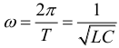
The period of harmonic oscillations in an electric oscillatory circuit is determined by the formula:

Cyclic frequency of oscillations in an electric oscillatory circuit:
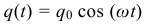
The dependence of the charge on the capacitor from time to oscillations in the electric circuit is described by the law:
The dependence of the electric current flowing through the inductor from time to time when oscillations in the electric circuit:

The dependence of the voltage on the capacitor from time to oscillations in the electric circuit:

The maximum value of the current during harmonic oscillations in an electric circuit can be calculated by the formula:

The maximum value of the voltage on the capacitor with harmonic oscillations in the electric circuit:

All real circuit comprise electric resistance R . The process of free oscillations in such a contour no longer obeys the harmonic law. For each period of oscillation, a part of the electromagnetic energy stored in the circuit is converted into heat generated on the resistor, and the oscillations become damped.
Alternating current. Transformer
Most of the electricity in the world is currently produced by alternating current generators that create sinusoidal voltage. They allow the simplest and most economical transmission, distribution and use of electrical energy.
A device designed to convert mechanical energy into alternating current energy is called an alternating current generator . It is characterized by an alternating voltage U ( t ) (induced by EMF) at its terminals. The operation of the alternator is based on the phenomenon of electromagnetic induction.
Alternating current is an electric current that varies over time according to a harmonic law. The values U 0 , I 0 = U 0 / Rare called the amplitude values of voltage and current. Values of voltage U ( t ) and current I ( t ) depending on time are called instantaneous .
Alternating current is characterized by the effective values of current and voltage. The effective (effective) value of an alternating current is called the strength of such a direct current, which, passing through the circuit, would produce the same amount of heat per unit of time as this alternating current. For alternating current, the effective value of the current can be calculated by the formula:

Similarly, you can enter the current (effective) value for voltage , calculated by the formula:

Thus, the expressions for DC power remain valid for alternating current, if we use in them the effective values of current and voltage:

Please note that if we are talking about voltage or AC power, then (unless otherwise stated) it is the actual value that is meant. So, 220V – is the current voltage in the home power supply.
AC capacitor
Strictly speaking, a capacitor does not conduct a current (in the sense that charge carriers do not flow through it). Therefore, if the capacitor is connected to the DC circuit, then the current strength at any time point at any point in the circuit is zero. When connected to the AC circuit due to a constant change in the EMF, the capacitor is recharged. The current through it still does not flow, but the current in the circuit exists. Therefore, conditionally they say that the capacitor conducts alternating current. In this case, the concept of capacitor resistance in an alternating current circuit (or capacitive impedance ) is introduced . This resistance is determined by the expression:

Note that the capacitance is dependent on the frequency of the alternating current. It is fundamentally different from the usual resistance of R. So, heat is released on resistance R (therefore, it is often called active), and heat is not released on capacitive resistance. The resistance is due to the interaction of charge carriers during the flow of current, and the capacitive – with the processes of recharging the capacitor.
Inductor in the AC circuit
When an alternating current flows in the coil, a phenomenon of self-induction arises, and, therefore, an emf. Because of this, the voltage and current in the coil do not coincide in phase (when the current is zero, the voltage has a maximum value and vice versa). Because of this mismatch, the average thermal power released in the coil is zero. In this case, the concept of coil resistance in an alternating current circuit (or inductive resistance ) is introduced . This resistance is determined by the expression:

Note that the inductive impedance depends on the frequency of the alternating current. Like capacitive impedance, it differs from resistor R. As with capacitive impedance, heat is not released on inductive impedance. Inductive resistance is associated with the phenomenon of self-induction in the coil.
Transformers
Among the devices of alternating current, which have found wide application in engineering, transformers occupy a significant place . The principle of operation of transformers used to raise or lower the AC voltage is based on the phenomenon of electromagnetic induction. The simplest transformer consists of a closed-core core on which two windings are wound: the primary and the secondary . The primary winding is connected to an alternating current source with a certain voltage U 1 , and the secondary winding is connected to a load on which a voltage U 2 appears . Here, if the number of turns in the primary winding is equal to n 1 , and secondary n2 , then the following relationship holds:

The transformation ratio is calculated by the formula:

If the transformer is ideal, then the following relationship holds (the input and output powers are equal):

The concept of efficiency is introduced in a non-ideal transformer:

Electromagnetic waves
To the table of contents …
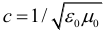
Electromagnetic waves – is an electromagnetic field propagating in space and in time. Electromagnetic waves are transverse – the vectors of electrical intensity and magnetic induction are perpendicular to each other and lie in a plane perpendicular to the direction of wave propagation. Electromagnetic waves propagate in a substance with a finite velocity, which can be calculated by the formula:

where: ε and μ are the dielectric and magnetic permeabilities of the substance, ε 0 and μ 0 are electric and magnetic constants: ε 0 = 8.85419 · 10 –12 F / m, μ 0 = 1.25664 · 10 –6 GN / m . The speed of electromagnetic waves in vacuum (where ε = μ = 1) is constant and equal to с = 3 ∙ 10 8 m / s, it can also be calculated by the formula:
The speed of propagation of electromagnetic waves in a vacuum is one of the fundamental physical constants. If an electromagnetic wave propagates in any medium, then its propagation velocity is also expressed by the following relationship:

where: n is the refractive index of a substance — a physical quantity that shows how many times the speed of light in a medium is less than in a vacuum. The refractive index, as can be seen from the previous formulas, can be calculated as follows:

- Electromagnetic waves carry energy. With the propagation of waves, a flow of electromagnetic energy occurs.
- Electromagnetic waves can be excited only by accelerated charges. DC circuits in which charge carriers move at a constant speed are not a source of electromagnetic waves. But the chains in which alternating current flows, i.e. such chains in which charge carriers constantly change their direction of movement, i.e. moving with acceleration – are a source of electromagnetic waves. In modern radio technology, the radiation of electromagnetic waves is produced using antennas of various designs, in which fast-alternating currents are excited.