Rational equations Formula
Rational equations are equations in which variables can be found in the denominators of rational expressions. 1 x + 1 = 2 x \dfrac{1}{x+1}=\dfrac{2}{x} x+11=x2start fraction, 1, divided by, x, plus, 1, end fraction, equals, start fraction, 2, divided by, x, end fraction is a rational equation.
Rational equation examples

A rational equation can be defined as an equation that involves at least one rational expression, or you can say a fraction. For example, 2x+14 = x3 is a rational equation. These fractions can be on one side or both sides of the equation.
Basic theoretical information
Abbreviated Multiplication Formulas
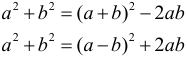
When performing various algebraic transformations, it is often convenient to use abbreviated multiplication formulas. Often these formulas are used not so much to shorten the multiplication process, but on the contrary, rather to see from the result that it can be represented as a product of some multipliers. Thus, these formulas need to be able to apply not only from left to right, but also from right to left. We list the basic formulas of abbreviated multiplication. Amount square:

Difference squared:

The previous two formulas are also sometimes written in a slightly different form, which gives us some kind of expression for the sum of squares:
You also need to understand what will happen if the characters in brackets in a square are placed in a “non-standard” way:

Now we go further. The formula for the abbreviated multiplication is the difference of the squares:

Cube difference:
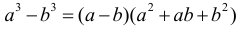
Sum of cubes:

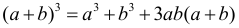
Amount Cube:

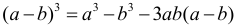
Difference Cube:

The latter two formulas are also often conveniently used in the form:
Quadratic equation and square triple
Let the quadratic equation be:

Then the discriminant is found by the formula:
If D > 0, then the quadratic equation has two roots, which are found by the formula :

If D = 0, then the quadratic equation has one root (its multiplicity: 2), which is sought by the formula :

If D <0, then the quadratic equation has no roots. In the case when a quadratic equation has two roots, the corresponding quadratic term can be factorized by the following formula :

If the quadratic equation has one root, then the decomposition of the corresponding square trinomial into factors is given by the following formula :
Only if the quadratic equation has two roots (that is, the discriminant is strictly greater than zero) the Viet theorem holds . According to the Vieta Theorem, the sum of the roots of a quadratic equation is:

The product of the roots of a quadratic equation according to the Viet theorem can be calculated by the formula:

The graph of a parabola is given by a quadratic function:

The coordinates of the vertex of the parabola can be calculated by the following formulas. X vertices (or the point at which the square trinomial reaches its highest or lowest value):

Parabola vertex game or maximum, if parabola branches are down ( a <0), or minimum, if parabola branches are up ( a > 0), the value of the square triple:

Basic properties of degrees
Mathematical degrees have several important properties, we list them. When multiplying degrees with the same bases, the exponents are added:
When dividing powers with the same bases, the divisor degree is subtracted from the exponent of the dividend:

When a degree is raised to a degree, the exponents are multiplied together:
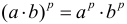
If numbers are multiplied with the same degree, but with different bases, then you can multiply the numbers first and then build the product to this power. The reverse procedure is also possible, if there is a product in the degree, then each of the multiplicated ones can be raised to this degree separately and the results multiplied:
Also, if numbers are divided with the same degree, but with different bases, then you can first divide the numbers, and then raise the quotient to this power (the inverse procedure is also possible):

Some simple degrees properties:


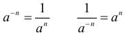
The last property holds only for n > 0. Zero can only be raised to a positive power. Well, the main property of the negative degree is written as follows:
Basic properties of mathematical roots
The mathematical root can be represented in the form of an ordinary degree, and then use all the properties of the degrees given above. To represent the mathematical root in the form of a degree, use the following formula:

Nevertheless, it is possible to write out separately a number of properties of mathematical roots, which are based on the properties of the degrees described above:


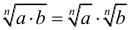

For arithmetic roots, the following property holds (which can also be considered the definition of a root):

The latter is true: if n is odd, then for any a ; if n is even, then only with nonnegative a . For the root of odd degree , the following equality is also fulfilled (from the root of the odd degree, one can remove the minus sign):

Since the value of a root of even degree can only be non-negative , for such roots there is the following important property:

Some additional algebra information
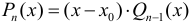
If x 0 is the root of a polynomial of the n- th degree P n ( x ), then the following equality holds (here Q n-1 ( x ) is some polynomial of the ( n – 1) th degree):
The procedure in which a square trinomial is represented as a bracket in a square and another term is called the selection of a complete square . And although the operation of allocating a full square is easier to perform each time “from zero” in concrete numbers, there is nevertheless a general formula with which you can write the result of the allocation of a complete square:

There is an operation inverse to the addition of fractions with the same denominators, and which is called term by division . It is that, on the contrary, each term from the sum in the numerator of a fraction should be written separately over the denominator of this fraction. For term operation, division can also be written the general formula:

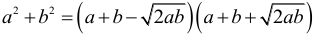
There is also a formula for factoring the sum of squares :
Solving rational equations
To solve an equation is to find all its roots. The main solution method is by algebraic transformations or change of variables to reduce the equation to an equivalent, which is solved simply (for example, to a square one). If the equation is not reduced to an equivalent, then secondary roots may arise. Doubt – check the roots by substitution.
For many equations, the concept of the domain of permissible values for the roots is important, then – the LDL. At this stage (in rational equations, ie, those that do not contain arithmetic roots, trigonometric functions, logarithms, etc.), the basic condition to which the roots of the equation must answer is that when they are substituted into the original form of the equation, the denominators of fractions did not go to zero, because it is impossible to divide by zero. Thus, the TLD includes all possible values except those that zero the denominators of the fractions.
When solving equations (and later on inequalities) it is impossible to reduce the factors with a variable in the left and right side of the equation (inequality), in this case you will lose the roots. It is necessary to transfer all the expressions to the left of the equal sign and put the “shrinking” factor out of the brackets; in the future, we must take into account the roots that it gives.
In order for the product of two or more parentheses to be zero, it is sufficient that each of them separately is zero, and the rest exist. Therefore, in such cases it is necessary in turn to equate all the brackets to zero. In the final answer, you need to write down the roots of all these “branches” of the solution (unless of course these roots are included in the LDL).
Sometimes some of the fractions in a rational equation can be reduced. It is necessary to try to do this and not to miss any such opportunity. But while reducing the fraction, you may lose the TLD, therefore, the fraction needs to be reduced only after writing the TCE, or at the end of the solution, substitute the obtained roots into the original equation to check for the existence of denominators.
So, to solve a rational equation it is necessary:
- Expand all denominators of all fractions into factors.
- Move all terms to the left to get a zero on the right.
- Record TLD.
- Reduce the fraction if possible.
- Lead to a common denominator.
- Simplify the expression in the numerator.
- Equate the numerator to zero and solve the resulting equation.
- Do not forget to check the roots for compliance with the TLD.
One of the most common methods for solving equations is the variable replacement method . Often, the replacement of variables is chosen individually for each specific example. It is important to keep in mind the two main criteria for introducing substitutions into equations. So, after introducing a replacement into some equation, this equation should:
- first, become simpler;
- secondly, no longer contain the original variable.
In addition, it is important not to forget to perform a reverse replacement, i.e. after finding the values for the new variable (for replacement), write instead of replacement for what it is equal through the original variable, equate this expression with the values found for replacement and again solve the equations.
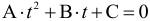
Separately, we dwell on the algorithm for solving very common homogeneous equations . Homogeneous equations are:

Here A, B and C are numbers that are not equal to zero, and f ( x ) and g ( x ) are some functions with variable x . Homogeneous equations are solved as follows: divide the entire equation by g 2 ( x ) and get:

Replace variables:

And solve the quadratic equation:
Having obtained the roots of this equation, we do not forget to perform the reverse replacement, and also to check the roots for compliance with the LDL.
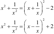
Also, when solving some rational equations, it would be good to remember the following useful transformations:
Solving systems of rational equations
To solve a system of equations means to find not just a solution, but sets of solutions, that is, such values of all variables that, being simultaneously substituted into the system, turn each of its equations into an identity. When solving systems of equations, the following methods can be applied (we don’t forget about DHS):
- Substitution method The method is to express one of the variables from one of the equations, substitute this expression for the unknown in the other equations, thus reducing the number of unknowns in the remaining equations. This procedure is repeated until one equation with one variable remains, which is then solved. The remaining unknowns are sequentially found by the already known values of the variables found.
- The method of splitting the system. This method consists in factoring one of the equations of the system. In this case, it is necessary that the right in this equation be zero. Then equating each factor of this equation in turn to zero and appending the remaining equations of the original system, we get several systems, but each of them will be simpler than the original one.
- The method of addition and subtraction. This method consists in adding or subtracting the two equations of the system (they can and often must be multiplied by a certain factor) to get a new equation and replace it with one of the equations of the original system. It is obvious that such a procedure makes sense only if the new equation will be obtained much simpler than the previously existing ones.
- The method of division and multiplication. This method consists in dividing or multiplying the left and right parts of the two equations of the system, respectively, to obtain a new equation, and replace it with one of the equations of the original system. It is obvious that such a procedure again makes sense only if the new equation will be obtained much simpler than the ones previously available.
There are other methods for solving systems of rational equations. Among which is the replacement of variables . Often, the replacement of variables is chosen individually for each specific example. But there are two cases where you always need to introduce a very specific replacement. The first of these cases is the case when both equations of a system with two unknowns are homogeneous polynomials equated to a certain number. In this case, you need to use a replacement:

After applying this replacement, by the way, it will be necessary to use the division method to continue solving such systems. The second case is symmetric systems with two variables, i.e. systems that do not change when replacing xwith y , and y with x . In such systems it is necessary to apply the following double change of variables:

At the same time, in order to introduce such a replacement into a symmetric system, the original equations will most likely have to be greatly transformed. Of course, we should not forget about the TLD and the obligatory implementation of reverse replacement in both of these methods.